Functional data structure are kind of a big deal, but what exactly makes them “functional”? After all, isn’t any data structure that works functional? Sorry, bad joke. In fact, a functional data structure is one that, like functional code itself, does not mutate state. Instead, functional data data structures are modified by copying the affected cells of a data structure and making changes in the copy. Okay you say, what does this buy me over a Vector?

To illustrate some of the advantages to functional data structures lets walk through the linked list. Linked lists are, as Chris Okasaki points out in his excellent book Purely Functional Data Structures, stacks. That is to say, you can add elements to the head of a list (push), or read off the head (pop). Both structures are head-optimized. So, what does a basic linked list implementation actually look like in Scala?

abstract class List_

case object Nil_ extends List_

case class Cons_[A](head: A, tail: List_) extends List_

object List_{
  def::[A](data: A, ls: List_) = Cons_(data, ls)

  def isEmpty(ls: List_) = ls match{
    case Nil_ => true
    case _ => false
  }

  def head(ls: List_) = ls match{
    case Cons_(h, t) => Some(h)
    case _ => None
  }

  def tail(ls: List_) = ls match{
    case Cons_(_, t: Cons_) => Some(t)
    case _ => None
  }
}

In fairly idiomatic Scala, you’ll start with a base interface List, then provide the empty case Nil. After that, every List is simply a bit of data added to the head of another List, aka Cons. Now lets imagine we want to append two lists together. With a mutable list you can just take the tail element of the list & set it as the head of the second list. However, with a functional list we don’t want to mutate the other list. So, how do we concatenate both lists without mutating either list?

def append(as: List_, bs: List_): List_ = as match{
    case Nil => bs
    case Cons_(h, t) => Cons_(h, append(t,bs))
  }

As you can see, instead of modifying either list I’ve walked both lists & constructed a third list from their elements. It’s the order of the traversal, from list A’s head -> list B’s tail that ensures the concatenation is in the correct order. There are a few other helper functions like foldLeft and reverse that we’ll need in a moment, so lets add them as well:

def foldLeft[T, A](ls: List_, seed: T)(f: (A, T)=> T): T =
    ls match{
      case Nil_ => seed
      case Cons_(h: A, t) => foldLeft(t, f(h, seed))(f)
      case _ => seed
    }

  def reverse[A](ls: List_) = ls match{
    case Nil_ => ls
    case Cons_(h:A, t) => foldLeft[List_, A](ls, Nil_)((x, seed) =>{
      seed match{
        case Nil_ => Cons_[A](h, Nil_)
        case Cons_(a:A, _) => Cons_[A](a, seed)
      }
    })
  }

Aside from the ugly syntax (easy enough to fix!) this should look somewhat similar to the standard library. Fold Left is still an eager tail-recursive fold, and reverse returns the same elements in opposite order.

Now that we have a solid linked list implementation, lets move one to creating everyone’s favorite FIFO structure, the queue.

Unlike stacks, which are great for parsing & similar algorithms, queues are well-suited for algorithms requiring time-ordering such as processing instructions in the order they were issued. In an imperative setting Queue’s are often implemented using an Array or Vector with pointers to the current head & tail held internally. However, since this implementation relies exclusively on mutation, it’s not going to suffice for our functional queue. Instead, we’ll implement the queue as a pair of lists. The following code illustrates how to construct a basic functional queue:

case class Queue_[A](f: List_, r: List_)

object Queue_{

  def isEmpty(q: Queue_[_]) = q match{
    case Queue_(Nil_, Nil_) => true
    case _ => false
  }

  def enQ[A](a: A, q: Queue_[A]) = Queue_(q.f, Cons_(a, q.r))

  def deQ[A](q: Queue_[A]): (Option[A], Queue_[A]) = {
    q match{
      case x if isEmpty(x) => (None, q)
      case Queue_(_Nil, x) => {
        val newF = List_.reverse(x)
        (List_.head(newF), Queue_(List_.tail(newF), Nil_))
      }
      case Queue_(f, r) =>
    }
  }

}

Now that’s certainly more interesting than just a plain linked list. Thanks to the extended List implementation I’m able to model the queue as two lists which swap places whenever the front (f) is empty. This means either enQ or deQ will be O(n) in the worst case since it will require a full traversal to preserve ordering. In my example, I chose to provide an O(1) insertion and leave O(n) worst case for removal. You’d need to profile or at least understand your workload better to determine whether this makes sense for a particular use case.

For more reading I really can’t recomend Chris Okasaki’s book enough, but Functional Programming In Scala is also a great resource. Good luck & feel free to send me an email with any questions.

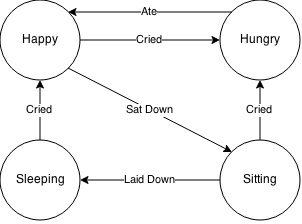
I’m assuming the reader is already familiar with finite state machines, otherwise I strongly recommend reading about them. Personally, I find them easiest to read as diagrams rather than tables or strings. For example, here’s a really simple diagram of a baby’s life:

Living the life...

Babies only have a couple of states: Happy, Hungry, Sitting on someone’s lap, or Sleeping. Different events may occur in the world that cause the baby to change states. Other events may not change the baby from one state to another, so the baby just continues along as it was.

Implementing this type of structure is really easy in Scala thanks to pattern matching & strong typing. Taking our baby example & translating it to code, we end up with this:

abstract class FsmState[T <: Enumeration](val state: T)

object BabyState extends Enumeration{
  type State = Value
  val Happy, Hungry, Sitting, Sleeping = Value
}
case class Baby(name: String, babyState: BabyState.State) extends FsmState(state =  babyState)

trait Event

case class Cried(id: String) extends Event
case class Ate(id: String) extends Event
case class Sat(id: String) extends Event
case class LaidDown(id: String) extends Event

object Baby{

  private def cloneNewState(d: Baby, s: BabyState.State) =
    d.copy(babyState = s)

  def transition(d: Baby, e: Event): Baby = {
    d.babyState match {
      case BabyState.Happy =>
        e match {
          case Cried(x) => cloneNewState(d, BabyState.Hungry)
          case Sat(x) => cloneNewState(d, BabyState.Sitting)
          case _ => d
        }
      case BabyState.Hungry =>
        e match {
          case Ate(x) => cloneNewState(d, BabyState.Happy)
          case _ => d
        }
      case BabyState.Sitting =>
        e match{
          case LaidDown(x) => cloneNewState(d, BabyState.Sleeping)
          case Cried(x) => cloneNewState(d, BabyState.Hungry)
          case _ => d
        }
      case BabyState.Sleeping =>
        e match{
          case Cried(x) => cloneNewState(d, BabyState.Happy)
          case _ => d
        }
      case _ => d
    }
  }

}

Okay, so that’s a little more than some circles & arrows, but hopefully not too difficult to look at. To start with, I’ve defined an abstract trait
<div class="highlight"><pre>FsmState[T <: Enumeration]</pre></div> which specifies that you’ll need to define a state enumeration & that the FSM state may only ever be in one state (pretty obvious). Next I define the basic case class to contain our state & have it extend <div class="highlight"><pre>FsmState[T <: Enumeration]</pre></div> .

Now that I have a domain object & some states, its time to build the actual state machine. Like I mentioned above, pattern matching on the Event classes make it incredibly simple to construct the full machine. First, you match on the current <div class="highlight"><pre>BabyState.State</pre></div> , then either allow a transition to a new state or drop through to the current state if no transition is allowed. Conversely you could return the error-handling type of your choice in the fall-through case.

This machine is trivially simple & doesn’t contain any business logic, but I’ll dive into how to add business logic to the transitions in the next post.

  • Special thanks to my 4-month old niece for the FSM inspiration.

Six months ago I decided to check out my first Haskell meetup at Akami’s Cambridge office. Seeing how everyone keeps singing Haskell’s praises and the meetup was only a block away I was locked in. After helping myself to the obligatory slice of pizza & bottle of water I sat down and cracked open my laptop, ready to take some notes & learn me some Haskell. The first talk was simple & understandable enough; a neuroscience PHD student had used Haskell to analyze his lab results & found the software transactional memory feature made concurrency easy for him. Between talks I congratulated myself for following his examples in such a mysterious language & even added What’s so confusing about this into my notes. The second talk flew way over my head, rapidly diving through Lambda Calculus (what’s that??) and moving into Inference Rules & Type Systems. Needless to say this talk left me reeling but motivated to learn what all of those Greek letters actually mean. The following post attempts to explain this to a liberal arts major like myself.

Lambda (λ) Calculus

Lambda Calculus is really little more than 8th grade algebra. It is based on the concepts of function abstraction - using variables to represent functions - and function application - assigning variable names to particular values. So while these concepts are very simple on the surface they are incredibly powerful and versatile. In fact, you can represent virtually any construct from any programming language as a lambda expression, which means any language could be represented purely via lambda expressions.

Function Abstraction

If you’re reading this then odds are you’re a programmer, have a passing interest in programming, or a friend of mine I conned into reading this. Regardless of your background, you probably remember learning in Pre-Algebra that 2x + 1 = y plots a straight line for any value of x and y. In that little example x & y are data variables that abstract away the x & y coordinates for an arbitrary point on the line. Function abstraction is what happens when we say f(x)=2x +1, so the equation for a line becomes f(x)=y. This abstraction has removed the concrete formula & provided a name in its place. This is the backbone of higher-order functions.

Function Application

Continuing with the example from above, f(x)=y gives us a lovely representation of our line, but ultimately we’re going to want to plot the line & to do that we’ll need to transform our formula into a series of (x,y) coordinates. The act of “specializing” a particular formula or expression by providing concrete values (in this case 2 _ +1) allows for eventual function evaluation. As you can see, abstraction & application work hand in hand.

λ Expressions

A λ expression is one of three things: a variable name identifying function abstraction, a non-abstracted function, or the application of a function. The BNF grammar would be:

Expression = Name | Function | Application
Function = λName.Body
Body = Expression
Application = (Function Argument)

For example λa.a λx.λy.y is a function that sets a variable a equal to the function λx.λy.y, which you can tell reduces to y. So the example statement reduces to y.

When evaluating a λ expression there are two possible approaches, applicative order and normal order. Applicative order means the parameter is evaluated before being passed into the function, while normal order means the parameter is evaluated after being passed in.

At this point you’re probably thinking “great, so I can write long convoluted λ expressions. There must be a cleaner way”. Thankfully, there is!

Beta (β) Reductions

β reductions is the formal name for replacing a particular λ function with a name. So, the β reduction of λa.a could be identity, since λa.a is the identity function in λ calculus. So really all we’ve done is take the concept of function abstraction discussed above & given it a fancy name & a Greek letter. Conceptually, this is the exact same as saying f(a) = a.

Alpha (α) Conversions

Now that we have the power to introduce abstraction at arbitrary places in our λ expressions, you’re probably concerned about naming collisions. After all, I could easily introduce a free variable with the same name as a bound variable, so how can I tell them apart? Thankfully α conversions enforce consistent renaming across all free instances of a variable. This is a complex name for the incredibly simple concept of choosing unique names for variables to avoid confusion.

Eta (η) Reductions

η reductions simplify an expression by removing unnecessary bound variables from the expression for instance, a statement *λa.(expr a) * will reduce to *expr * via an η reduction. This process strips out unnecessary variables from a λ expression to clarify the meaning.

In no way have I attempted to provide a comprehensive overview of λ calculus, but I do hope this gives people enough information to prevent them from being completely lost whenever these terms pop up in conversation. Thanks for reading and please contact me with any questions or corrections.